What is cluster analysis?
Cluster analysis is a data analysis technique that explores the naturally occurring groups within a data set known as clusters. Cluster analysis doesn’t need to group data points into any predefined groups, which means that it is an unsupervised learning method. In unsupervised learning, insights are derived from the data without any predefined labels or classes. A good clustering algorithm ensures high intra-cluster similarity and low inter-cluster similarity.
An example of a data clustering problem
Grouping retail outlets based on their sales is a simple use case of clustering analysis. Assume that a café has eight outlets in the city. The table below shows the sales of cappuccino and iced coffee per day.
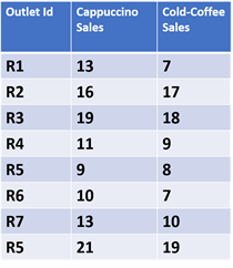
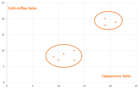
The graph below shows the same data where cappuccino and iced coffee sales for each outlet are plotted on the X and Y axes, respectively. In this example, as there were limited data points, it was easy to plot the two naturally occurring clusters of café outlets on a graph and visualize them manually.
However, when it comes to thousands of data points, cluster analysis algorithms need to be used to segregate the data points into different clusters.
What are the applications of cluster analysis?
Cluster analysis is often used in two main ways:
- As a stand-alone tool for solving problems related to data grouping.
- As a pre-processing step for various machine learning algorithms.
Cluster analysis as a stand-alone tool
- Marketing: In marketing, cluster analysis can be used to segregate customers into different buckets based on their buying patterns or interests. These are known as customer personas. Organizations then use different marketing strategies for different clusters of customers.
- Risk Analysis in Finance: Financial organizations use various cluster analysis algorithms for segregating their customers into various risk categories based on their bank balance and debt. While approving loans, insurance, or credit cards, these clusters are used to aid in decision-making.
- Real Estate: Infrastructure specialists use clustering to group houses according to their size, location, and market value. This information is used to assess the real estate potential of different parts of a city.
Cluster analysis as a pre-processing step for machine learning
Cluster analysis is often used as a pre-processing step for various machine learning algorithms.
Classification algorithms run cluster analysis on an extensive data set to filter out data that belongs to obvious groups. Advanced data classification techniques can then be used on the reduced, non-obvious data points. As the data set becomes smaller, computation time is highly reduced. The same method can be used in the opposite way, where a cluster analysis algorithm is used to filter out the noise or outlier data.
Before running a supervised learning algorithm, one might first do cluster analysis on the input data to find out the natural clusters in the data.
What are the major cluster analysis algorithms?
Cluster analysis algorithms often belong to the following categories:
- Partition-based algorithms
- Hierarchical algorithms
- Density-based algorithms
- Grid-based algorithms
- Model-based algorithms
- Constraint-based algorithms
- Outlier analysis algorithms
Each algorithm is complex within itself and may be suitable for some analyses and not others.
Partition-based algorithms for cluster analysis
In this method, an algorithm starts with several initial clusters. Then it iteratively relocates the data points to different clusters until an optimum partition is achieved. K-means clustering algorithm is one of the most popular clustering algorithms.
A K-means clustering example below shows how this works.What Are the Applications of Cluster Analysis?
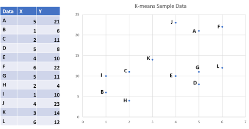
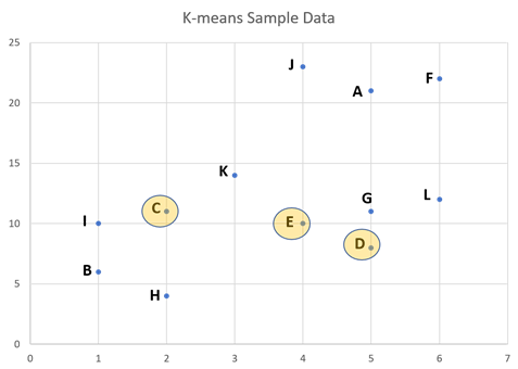
Step 1: Decide on clusters
Decide the number of clusters, “K” for the algorithm, for example, K=3. The algorithm will partition the above twelve data points into 3 clusters. The number K can be any value. Depending on that, the correctness of the clustering may vary. There are also algorithmic methods that can be used to determine the optimal value for K.
Step 2: Choose data points
As K=3, take any three data points as the initial means. In this example, points C, D, and E are chosen as the initial means. Note that the K-means algorithm can take any point as the initial mean.
Step 3: Calculate the distances
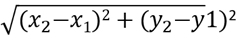
Calculate the distance from every point in the data set to each initial cluster mean. Three cluster-means C, D, and E have randomly been chosen. For each data point in the sample, calculate it’s the distance from these three means. The Euclidean distance between two points (X1, Y1) and (X2, Y2) is used as below:
After step 3, a table would show the distance of each data point from the initial means C, D, and E.
A data point is added to a cluster based on its minimum distance. For example, point A has a minimum distance from an initial mean C. This means that A is in the cluster with mean as C. After the first step, the clusters are obtained.
Step 4: Reiteration – Calculation of New Means
Now it is easy to see the initial clusters. The next step is to calculate three new cluster means. For this, every data point in a particular cluster is taken, and a mean is calculated.
New cluster mean for the “C” cluster = (5+2+6+1+4+3+6/7, 21+11+22+10+23+14+12/7) = (3.85, 16.14), Let’s call this point X.
New cluster mean for the “D” cluster = (1+2+5/3, 6+8+4/3) = (2.66, 6), Let’s call this point Y.
New cluster mean for the “E” cluster = (4+5/2, 10+11/2) = (4.5, 10.5). Let’s call this point Z.
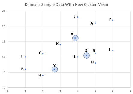
Step 5: Reiteration—Calculate the distance of each data point from the new means
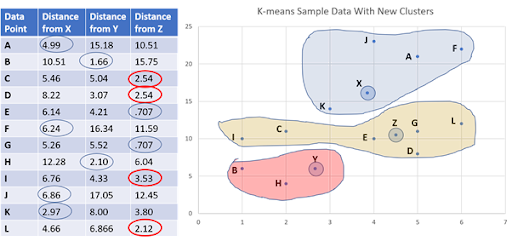
Repeat step 3 to find out the distance of all data points from the newly calculated cluster means, X, Y, and Z. In this new iteration, it is easy to see that the minimum distance of the data points C, D, I, and L has changed. They now belong to a new cluster, as shown below.
Then, the K-means iteration needs to continue as some of the data points have changed their clusters.
Step 6: Reiteration—Calculation of New Means and New clusters
As the data points C, D, I, L have changed their clusters, new cluster means need to be calculated as in step 4. For this, every data point in a particular cluster is taken, and an average is calculated. Then like in step 5, the distance from each data point to the new cluster mean is calculated. Based on the distance, the data points are assigned to a cluster to which it has a minimum distance.
When does the K-means algorithm finish?
K-means is an iterative partition algorithm:
- Decide the number of clusters(K) to start with. In the above example, K=3.
- Randomly assign K number of data points as the initial cluster means.
- Repeat the below steps till no data point changes its cluster.
- Calculate mean distance from the data point to cluster mean.
- Assign a data point to the cluster with the lowest distance.
- Check if any data point has changed its cluster.
In a new iteration, if every data point remains in its previous cluster, the K-means algorithm terminates. This means a locally optimum solution has been obtained.
K-medoid partition-based clustering algorithm
K-medoids algorithm is another partition-based clustering algorithm. The K-medoid algorithms choose medoids as a representative object of a cluster. The K-medoid algorithm tries to find such data points that have a minimum dissimilarity from every other data point in a particular cluster. Until the dissimilarity is minimized, the K-medoid algorithm iteratively partitions the data set. K–means algorithm often uses squared error distance (Euclidean distance), and K–medoid algorithms often use absolute value distance like Manhattan distance to measure dissimilarity between two data points.
A standard implementation of the K–medoid algorithm is Partition Around Medoids (PAM) algorithm. Here are the basic steps of the PAM algorithm.
- Choose a value for K, where K is the number of clusters into which the data points will be divided.
- Choose K number of data points randomly as medoids.
- For every data point (Xi, Yi) in the data set, measure the dissimilarity between the point and the above-selected medoids. An often-used measure for dissimilarity is the Manhattan distance:
- | Xi – Ci| + | Yi - Cj|, where (Ci, Cj) represents a medoid.
- Each data point (Xi, Yi) is assigned to a cluster where dissimilarity is minimal.
- For each of the above clusters, calculate the total cost – the sum of the dissimilarities of each of the data points in that cluster.
- Now, randomly select a non-medoid point to be the new medoid and repeat steps 3-5.
- Stop when there are no changes in the clusters.
Comparison of K-means and K-medoid algorithms
Even though the K- means algorithm is simple, it doesn’t produce good results when the data has a lot of noise and outliers. The K-medoid method is more robust in such cases. However, the K-medoid algorithms like PAM are only useful when the data set is small. When the data set size increases, the computation time for the K -medoid algorithm exponentially increases.
Divisive algorithms
As the name suggests, divisive algorithms assign all the data points into a single cluster in the beginning. It then divides the cluster into least similar clusters. The algorithm then recursively divides these clusters until an optimum solution is achieved. Divisive algorithms are also known as a top-down clustering method.
Agglomerative algorithms
These algorithms start with assigning each data point to a different cluster. Then, the algorithm recursively joins the most similar clusters until an optimum solution is achieved. Agglomerative algorithms are also known as the bottom-up clustering method.
Example of an Agglomerative Clustering Algorithm
Below is a distance matrix for five data points. The distance between the points can be calculated based on Euclidean distance or Manhattan distance or any other distance formula. The distance matrix is always a symmetric matrix, as the distance between points X and Y is the same as that between Y and X. Based on this distance matrix, an example of an agglomerative (bottom-up) clustering algorithm.
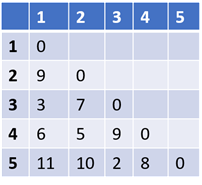
Step 1: In the distance matrix, find the two points whose distance is the smallest. In the above example, it is points 3 and 5. The distance between them is 2. Put them into a single cluster.
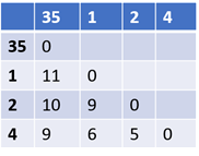
Step 2: Remove points 3 and 5 and replace it with a cluster “35” and create a new distance matrix. For this, the distance between all data points and the cluster “35” needs to be calculated. There are various ways to determine this distance.
In this example, the following method has been used to measure the distance:
Distance of point X from cluster “35” = minimum (distance (X, 3), distance(X,5)). The updated distance matrix based on this method is:
Step 3: Repeat step 2 until all the data points are grouped into one cluster. In the current example, it takes six iterations. The below diagram shows the formation of clusters. This kind of representation is known as a dendrogram. In this representation, the Y-axis represents the distance between two data points. For example, the distance between points 3 and 5 is 2.
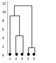
Step 4: Once all the data points are clustered, as shown above, decide how many clusters need to be retained. It’s a tough decision because every hierarchical clustering algorithm finally yields a single cluster. There are several methods available for deciding the optimum number of clusters after a hierarchical clustering algorithm partitions the data.
Density-based clustering algorithms
These algorithms are based on the idea that clusters are always denser than their surrounding data space. Density-based algorithms start with a single data point and explore the data points in its neighborhood. The points in the neighborhood of the initial point are included in a single cluster. The definition of neighborhood varies depending on the implementation of the algorithm. Density-based spatial clustering of applications with noise (DBSCAN) is a popular clustering algorithm in this category.
Grid-based clustering algorithms
Grid-based clustering algorithms are similar to the density-based ones. The data space is divided into several smaller units known as grids. Each data point is assigned to a particular grid cell. The algorithm then computes the density of each grid. Those grids whose density is lower than a threshold are eliminated. Next, the algorithm forms clusters from adjacent groups of dense grids. Statistical information grid (STING) and clustering in quest (CLIQUE) are two popular grid-based algorithms.
In addition to the above-discussed algorithms, clustering analysis includes a group of model-based clustering, constraint-based clustering, and outlier analysis algorithms.
Advantages and disadvantages of clustering analysis algorithms
| Algorithm | Advantages | Disadvantages |
|---|---|---|
| Partition-based cluster analysis algorithms |
|
|
| Hierarchical cluster analysis algorithms |
|
|
| Density-based cluster analysis algorithms |
|
|
| Grid-based cluster analysis algorithms |
|
|